Kodlama Pratiği
# This Python 3 environment comes with many helpful analytics libraries installed
# It is defined by the kaggle/python docker image: https://github.com/kaggle/docker-python
# For example, here's several helpful packages to load in

import numpy as np # linear algebra
import pandas as pd # data processing, CSV file I/O (e.g. pd.read_csv)
import seaborn as sns
import matplotlib.pyplot as plt
# import warnings
import warnings
# filter warnings
warnings.filterwarnings('ignore')

# Input data files are available in the "../input/" directory.
# For example, running this (by clicking run or pressing Shift+Enter) will list the files in the input directory

# Any results you write to the current directory are saved as output.
Veri Setini Yükleme
- MNIST verisetini kullanacağız (https://www.kaggle.com/competitions/digit-recognizer).
- Bu bölümde verileri yüklüyor ve görselleştiriyoruz.
# read train
train = pd.read_csv("train.csv")
print(train.shape)
(42000, 785)
# read test
test= pd.read_csv("test.csv")
print(test.shape)
(28000, 784)
# put labels into y_train variable
Y_train = train["label"]
# Drop 'label' column
X_train = train.drop(labels = ["label"],axis = 1)
# visualize number of digits classes
plt.figure(figsize=(15,7))
g = sns.countplot(Y_train, palette="icefire")
plt.title("Number of digit classes")
Y_train.value_counts()
1    4684
7    4401
3    4351
9    4188
2    4177
6    4137
0    4132
4    4072
8    4063
5    3795
Name: label, dtype: int64

# plot some samples
img = X_train.iloc[0].values
img = img.reshape((28,28))
plt.imshow(img,cmap='gray')
plt.title(train.iloc[0,0])
plt.axis("off")
plt.show()

# plot some samples
img = X_train.iloc[3].values
img = img.reshape((28,28))
plt.imshow(img,cmap='gray')
plt.title(train.iloc[3,0])
plt.axis("off")
plt.show()

Normalization, Reshape and Label Encoding
- Normalization
- Aydınlatma farklılıklarının etkisini azaltmak için gri tonlamalı bir normalizasyon gerçekleştiriyoruz.
- Normalizasyon yaparsak CNN daha hızlı çalışır.
- Reshape
- Eğitim ve test görüntüleri (28 x 28)
- Tüm verileri 28x28x1 3D matrislere yeniden şekillendiriyoruz.
- Keras'ın sonunda kanallara karşılık gelen ekstra bir boyuta ihtiyacı var. Görüntülerimiz gri ölçeklidir, bu nedenle yalnızca bir kanal kullanır.
- Label Encoding
- Etiketleri bir hot vectore kodlayın
- 2 => [0,0,1,0,0,0,0,0,0,0]
- 4 => [0,0,0,0,1,0,0,0,0,0]
- Etiketleri bir hot vectore kodlayın
# Normalize the data
X_train = X_train / 255.0
test = test / 255.0
print("x_train shape: ",X_train.shape)
print("test shape: ",test.shape)
x_train shape:  (42000, 784)
test shape:  (28000, 784)
# Reshape
X_train = X_train.values.reshape(-1,28,28,1)
test = test.values.reshape(-1,28,28,1)
print("x_train shape: ",X_train.shape)
print("test shape: ",test.shape)
x_train shape:  (42000, 28, 28, 1)
test shape:  (28000, 28, 28, 1)
# Label Encoding
from keras.utils.np_utils import to_categorical # convert to one-hot-encoding
Y_train = to_categorical(Y_train, num_classes = 10)
Train Test Split
- Verileri eğitim ve test kümelerine ayırıyoruz.
- Test boyutu %10'dur.
- eğitim boyutu %90'dır.
# Split the train and the validation set for the fitting
from sklearn.model_selection import train_test_split
X_train, X_val, Y_train, Y_val = train_test_split(X_train, Y_train, test_size = 0.1, random_state=2)
print("x_train shape",X_train.shape)
print("x_test shape",X_val.shape)
print("y_train shape",Y_train.shape)
print("y_test shape",Y_val.shape)
x_train shape (37800, 28, 28, 1)
x_test shape (4200, 28, 28, 1)
y_train shape (37800, 10)
y_test shape (4200, 10)
# Some examples
plt.imshow(X_train[2][:,:,0],cmap='gray')
plt.show()

Keras ile Uygulama
Modeli Oluşturma
- conv => max pool => dropout => conv => max pool => dropout => fully connected (2 katman)
- Dropout (Unutturma): Dropout, eğitim sırasında rastgele seçilen nöronların göz ardı edildiği bir tekniktir.
- Bir modelin aşırı öğrenmesini önlemek için kullanılır.

#
from sklearn.metrics import confusion_matrix
import itertools

from keras.utils.np_utils import to_categorical # convert to one-hot-encoding
from keras.models import Sequential
from keras.layers import Dense, Dropout, Flatten, Conv2D, MaxPool2D
from keras.optimizers import RMSprop,Adam
from keras.preprocessing.image import ImageDataGenerator
from keras.callbacks import ReduceLROnPlateau

model = Sequential()
#
model.add(Conv2D(filters = 8, kernel_size = (5,5),padding = 'Same', activation ='relu', input_shape = (28,28,1)))
model.add(MaxPool2D(pool_size=(2,2)))
model.add(Dropout(0.25))
#
model.add(Conv2D(filters = 16, kernel_size = (3,3),padding = 'Same', activation ='relu'))
model.add(MaxPool2D(pool_size=(2,2), strides=(2,2)))
model.add(Dropout(0.25))
# fully connected
model.add(Flatten())
model.add(Dense(256, activation = "relu"))
model.add(Dropout(0.5))
model.add(Dense(10, activation = "softmax"))
Optimizer'ı Tanımla
- Adam optimizer: Öğrenme oranını değiştirin.
# Define the optimizer
optimizer = Adam(lr=0.001, beta_1=0.9, beta_2=0.999)
Compile Model
- categorical crossentropy
- Önceki bölümlerde ve makine öğrenimi dersinde binary crossentropy yapıyoruz
- Şu anda categorical crossentropy kullanıyoruz. Bu, çoklu sınıfımız olduğu anlamına gelir.

# Compile the model
model.compile(optimizer = optimizer , loss = "categorical_crossentropy", metrics=["accuracy"])
WARNING:tensorflow:From C:\ProgramData\Anaconda3\lib\site-packages\keras\optimizers.py:790: The name tf.train.Optimizer is deprecated. Please use tf.compat.v1.train.Optimizer instead.

WARNING:tensorflow:From C:\ProgramData\Anaconda3\lib\site-packages\keras\backend\tensorflow_backend.py:3295: The name tf.log is deprecated. Please use tf.math.log instead.
Epochs and Batch Size
- Diyelim ki 10 örnekten (veya numuneden) oluşan bir veri kümeniz var. 2'lik bir batch size sahipsiniz ve algoritmanın 3 epoch boyunca çalışmasını istediğinizi belirttiniz. Bu nedenle, her bir epoch'ta 5 batch (10/2 = 5) vardır. Her parti algoritmadan geçer, bu nedenle epoch başına 5 iterasyonunuz olur.
- referans: https://stackoverflow.com/questions/4752626/epoch-vs-iteration-when-training-neural-networks
epochs = 10  # for better result increase the epochs
batch_size = 250
Data Augmentation
- Aşırı uyum sorununu önlemek için, el yazısı rakam veri setimizi yapay olarak genişletmemiz gerekir
- Rakam varyasyonlarını yeniden üretmek için eğitim verilerini küçük dönüşümlerle değiştirin.
- Örneğin, sayı ortalanmamıştır Ölçek aynı değildir (bazıları büyük/küçük sayılarla yazar) Görüntü döndürülmüştür.
*

# data augmentation
datagen = ImageDataGenerator(
        featurewise_center=False,  # set input mean to 0 over the dataset
        samplewise_center=False,  # set each sample mean to 0
        featurewise_std_normalization=False,  # divide inputs by std of the dataset
        samplewise_std_normalization=False,  # divide each input by its std
        zca_whitening=False,  # dimesion reduction
        rotation_range=0.5,  # randomly rotate images in the range 5 degrees
        zoom_range = 0.5, # Randomly zoom image 5%
        width_shift_range=0.5,  # randomly shift images horizontally 5%
        height_shift_range=0.5,  # randomly shift images vertically 5%
        horizontal_flip=False,  # randomly flip images
        vertical_flip=False)  # randomly flip images

datagen.fit(X_train)
Fit the model
# Fit the model
history = model.fit_generator(datagen.flow(X_train,Y_train, batch_size=batch_size),
                              epochs = epochs, validation_data = (X_val,Y_val), steps_per_epoch=X_train.shape[0] // batch_size)
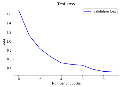
Modeli Değerlendirme
- Test Kaybı görselleştirme
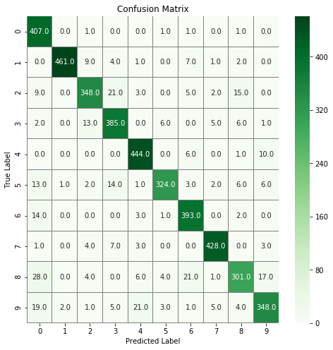
- Confusion matrix (karmaşıklık matrisi)
# Plot the loss and accuracy curves for training and validation
plt.plot(history.history['val_loss'], color='b', label="validation loss")
plt.title("Test Loss")
plt.xlabel("Number of Epochs")
plt.ylabel("Loss")
plt.legend()
plt.show()
# confusion matrix
import seaborn as sns
# Predict the values from the validation dataset
Y_pred = model.predict(X_val)
# Convert predictions classes to one hot vectors
Y_pred_classes = np.argmax(Y_pred,axis = 1)
# Convert validation observations to one hot vectors
Y_true = np.argmax(Y_val,axis = 1)
# compute the confusion matrix
confusion_mtx = confusion_matrix(Y_true, Y_pred_classes)
# plot the confusion matrix
f,ax = plt.subplots(figsize=(8, 8))
sns.heatmap(confusion_mtx, annot=True, linewidths=0.01,cmap="Greens",linecolor="gray", fmt= '.1f',ax=ax)
plt.xlabel("Predicted Label")
plt.ylabel("True Label")
plt.title("Confusion Matrix")
plt.show()